By Martin Pavlíček
Motivation
We set out to analyze various optimization techniques in a more controlled and simpler environment for the sake of better understanding the parallelization paradigms and to be leveraged in further Space Engineers development. As an environment, we chose Manual Badger (original source code) written by Marek Rosa, which was simple enough to quickly iterate and see the results. As we started, Manual Badger was already written using data oriented design and naively parallelized. Our goal was to improve performance to better leverage multi core CPUs, namely by reduction of sync points (Chapter 1), improvement of cache coherency (Chapter 2) and ultimately using massive parallelism via GPGPU (Chapter 3).
Some of the steps will change the outcome of the simulation slightly, which we have not addressed properly for the sake of simplicity.
In the previous chapter we’ve more or less saturated the compute capabilities of our test CPUs and even through significant effort our attempts to improve either single-threaded throughput or multi-threaded scaling of our code were met only with diminishing returns. For this reason, we’ve decided to explore different kinds of hardware to see if we could possibly gain some performance there.
GPUs are notoriously known for their massive parallelism capabilities and GPGPU computing is on a steep rise lately due to their compute throughput superiority to the CPUs so in this chapter we’ll try to adapt the Badger algorithm for GPUs to see if/how much we could benefit from alternative compute HW.
Source Code
The source code with ILGPU implementation is available here.
Overview
All data available here: Hardware Runoffs
| Compute device | Runtime | Relative speedup | |
| Vanilla badger | i7 9700K | 17,650 ms | 1x |
| Chapter 1 | i7 9700K | 3,394 ms | 5.20x |
| Chapter 2 | i7 9700K | 980 ms | 18.01x |
| GPU port | RTX 2060 | 2,967 ms | 5.95x |
| Asynchronous computation | RTX 2060 | 432 ms | 40.86x |
| Optimized data access | RTX 2060 | 312 ms | 56.57x |
| Data layout | RTX 2060 | 192 ms | 91.93x |
| Precompiled launch | RTX 2060 | 139 ms | 126.98x |
| Coalesced data access | RTX 2060 | 98 ms | 180.10x |
| Segmented updates | RTX 2060 | 19 ms | 928.95x |
| Large dataset (16x) | i7 9700K | 31,434 ms | 8.98x (1x) |
| Large dataset (16x) | RTX 2060 | 262 ms | 1077.86x (123.79x) |
Table 1: Time for 5K iterations of the Badger algorithm
GPU adaptation
There are multiple ways to get the Badger code on GPU ranging from handwritten HLSL shaders, that would mirror the Badger logic and executing them via DirectCompute API, to generating GPU code from high-level language like C# using cross compilers and executing it by target/platform-specific APIs/runtimes.
The former approach needs quite a lot of boilerplate code on the CPU side, requires knowledge of additional language to write the compute shader itself and all data structures and shared logic needs to be duplicated in the compute shader. The advantage of the DirectCompute is that it is mostly compatible across a multitude of (gaming) platforms.
The latter approach allows the programmer to focus on the algorithm at hand instead of context switching between two languages and code bases that need to cooperate, thus eliminating an entire range of nasty bugs and ensuring faster iterations. Done correctly, one can write GPU and CPU code in a “single source” manner (See Code snippet 1) and fluently transfer data and control-flow between the compute contexts/devices without being hindered by foreign compute API and desyncs in shared logic and data structure layouts.
struct PhysicBody
{
    public Vector3 Position;
    public Vector3 Velocity;
}
Task IntegrateBodies(Span bodies, float time)
{
    if (UseGPUAcceleration())
    {
        return GPU.ParallelFor(bodies.Length, i => IntegratePhysicBody(i, bodies, time));
    }
    else
    {
        return Parallel.For(bodies.Length, i => IntegratePhysicBody(i, bodies, time));
    }
}
//This is plain compute function that can run on CPU or GPU
void IntegratePhysicBody(int index, Span bodies, float time)
{
    bodies[index].Position += bodies[index].Velocity * time;
}
Code snippet 1: Example of C# driven GPGPU
While it sounds great, the compilers and tooling are unfortunately not yet on the level where we would like or need it to be – especially in regards to cross-platform support. The field is young though, lots of new compilers are being developed and the holes in tooling are being filled up gradually. HW (vendors) and driver APIs typically don’t differ much in terms of raw performance, usually the only significant differences come in naming scheme, feature set, and (cross) platform support. Due to limited cross platform options of both compilers and driver APIs we’ll measure only one HW vendor and only one driver API, though all optimization techniques used in this chapter as well as final performance measurements are applicable across different driver APIs/runtimes (Vulkan compute, OpenCL, DirectCompute, …) and major HW vendors (NVIDIA and AMD). Should our tests prove the GPGPU to be usable in real applications and bring significant performance improvements to the table, only then we’ll invest more time into exploring more cross-platform solutions.
As for the test HW, we’ll roll with NVIDIA; according to the Steam HW survey, it’s currently the major GPU vendor with close to 75% market share. With a broad feature set, extensive documentation, tooling and state-of-the-art HW abstraction, NVIDIACuda™ is a natural driver API of choice for our tests. NVIDIA Nsight Compute™ will then be used for all HW measurements and performance profiling.
While modern gaming CPUs feature 4, 8, 16, or up to 32 hardware threads, modern gaming GPUs can host anywhere from 10368 (GTX 1050) to 83968 (RTX 3090) hardware threads and application is expected to use all of them in order to fully saturate the hardware. This means that the threading model used in the previous chapters, where one thread processed an entire line, is no longer applicable as we simply don’t have that many lines in the data set to saturate the hardware.
In the Badger data set there are 65536 individual cells which is roughly enough to fully saturate our testing GPU, the RTX 2060 (30720 HW threads), if we adjust the threading model in a way that every thread gets assigned exactly one cell and run as many threads in parallel as possible, considering the cross-cell interference.
Copying data from RAM to GPU, running all 3 phases of Badger on GPU and then copying results from GPU back to RAM (in lock-step manner) yields a runtime of 2967ms for 5K iterations. Considering this is absolutely terrible usage of the HW (read further), we still beat the best CPU times from Chapter 1 by ~15%, it’s a very solid start indeed.
Asynchronous computation
Naturally, it is not very efficient to stall the CPU for the duration of the GPU computation. They are independent devices after all and can perform their computations concurrently and asynchronously. Standard GPGPU compute model assumes that the CPU only prepares work and data for the GPU and proceeds with other work, leaving the GPU to do the rest without any additional CPU participation. When the GPU is done with the work the CPU will collect results later during the frame (or during subsequent simulation frames), thus achieving minimal/no CPU stalls. Furthermore, GPUs can simultaneously perform computation work and memory transfers which (along with DMA) ensures that, when scheduled correctly, data transfers come at no cost on either of the compute devices.
Assuming our algorithm meets this criteria, we can remove the CPU <-> GPU synchronization overhead entirely in our benchmark by scheduling 5K iterations of the Badger algorithm for the GPU without waiting for each iteration to finish first and measuring the time it takes for the GPU to crunch through all of it and deliver the final results back to RAM. This results in a very favorable runtime of 432ms. At this point, our mid-end RTX 2060 card beats the best times of high-end i7-9700K CPU from Chapter 2 by a factor of 2x, still without any GPU-specific optimizations.
Optimized data access
As mentioned above, GPUs can host quite a substantial amount of HW threads, but it comes at a cost. Compared to CPU threads, GPU threads have only a limited number of registers, no stack, and very limited cache, so data need to be reloaded more often from GPU’s main memory, caches are evicted frequently and prefetching is non-existent. There is also no out-of-order execution (pipelining is present) so it’s harder to hide latencies of individually expensive instructions.
This is especially painful in phase 3 of the Badger algorithm where there is a lot of local state (increased register pressure) and threads probe a wide range of neighbor cells to finish the computation, thus hitting a lot of cache misses and loads from global memory with high latencies. This is not such an uncommon issue though and there is a well-known optimization procedure to address it.
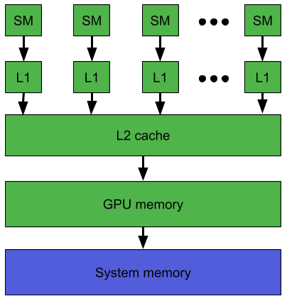
High-level onboard memory hierarchy is practically identical for all modern GPUs. Large global memory in remote chips, shared L2 cache close to compute chip and small L1 cache next to every compute core (streaming multiprocessor in case of team green), sorted by decreasing latency and increasing bandwidth. GPU compute kernels can manage the L1 cache on their own and allocate memory segments in the L1 for custom use. This means that we can spatially split the threads for phase 3 into work groups of 16×16 cells, download all cells needed for this block into the L1 cache first, and then reuse this cached data across all threads that participate in the computation of this block. This will reduce the number of times each cell needs to be read from the main memory by 24x, decreasing both total data transfer required for each iteration as well as latencies of each read by decreasing pressure on the global memory system. Runtime after this optimization improves to 312ms as a result.
Data layout
Now with the memory optimizations in place, we’re still bound on memory, how is that? Even more so, we’re bound by the memory subsystem but theoretical memory bandwidth is by far not fully utilized according to the profiler.
GPU memory is optimized for throughput, but not necessarily for latency. This is usually not an issue when there are enough threads that can saturate the compute cores while other threads wait for memory fetches to finish. This is not our case though, as all Badger phases start with a number of uncoalesced (thus expensive) reads followed by a pretty minimal amount of compute work which can be finished way faster than next batch of memory fetches finish, resulting in under-utilized/starving compute cores.
All Badger phases start with reads of 4 important fields, Cell Type, Gender, MovedThisFrame, and Age). These allocate one int (32 bits) each in the Cell structure even though they effectively utilize no more than 8 bits each. By packing these 4 values into consecutive 32 bits (8b per field) we can fetch them in a single memory request and reduce the number of global memory reads by up to 4x in exchange for a very small compute overhead caused by newly introduced unpacking. Compute cores are currently underutilized anyway so the cost is minimal. Furthermore, Cell structure size drops to 32 Bytes after this change, which is an aligned value and the compiler can start using fused memory loads and stores, which can transfer up to 128bits in a single request. This will be especially useful for phase 2 where we move entire Cells. Instead of 11 x 32 bit requests, we now need to perform only 2 x 128 bit transfers to move an entire cell. Runtime after this optimization comes down to 192ms.
Precompiled launch graph
At this point we’re flooding the driver, PCI-E bus and GPU itself with thousands of kernel launches each second. While not really a problem, it’s not optimal either as each separate launch comes with some small overhead. Since we know precisely the number and order of launches that are required for each iteration, we can precompile a launch graph for the entire iteration and start the whole iteration with a single driver call. This will reduce the CPU workload needed to submit the work on both the app and driver side as well as give the driver additional opportunity to optimize the launches on the GPU itself (mainly related to context switching on the HW side). The final runtime after this optimization is 139ms.
Coalesced data access
According to the profiler we’re still overwhelmingly bound on the memory subsystem, though still with only ~50% bandwidth utilization and compute cores utilization at 15-20%. This is mainly due to the large number of small uncoalesced memory reads that are dominating the algorithm with large latencies and preventing effective utilization of the available GPU compute capacity. The usual way to address this is to convert the data structures from AoS to SoA format (https://en.wikipedia.org/wiki/AoS_and_SoA) so that the memory reads are maximally coalesced across thread warps, achieving higher effective bandwidth utilization and smaller latencies at the same time.
In order to further reduce the memory system pressure, we’ll pack the commonly used fields more tightly into consecutive 32bits (Age 8b; LSA 8b; Gender 4b; Type 4b; MtF 8b) to get better memory coherency. In the SoA style, we’ll then get one array of tightly packed cell info that thread warps can access and read sequentially without wasting bandwidth on unused data, thus getting much lower latency, and the second array will be then allocated for larger data like `TraitsOrPreferences` that are used only sparsely throughout the simulation. With these optimizations the runtime drops further to 98ms.
Segmented updates
Currently, we run Badger phases one after another in separate compute kernels with sync points between them, iteration after iteration. This also means that we have to (re)load cell data at the beginning of every phase. Profiler claims that these loads are the most expensive part of the compute kernels, mainly due to high cache miss rates on these reads.
In the previous chapter we’ve discovered that cache hit rates improve considerably if we slice up the updates into small segments and do all phases in one go (as opposed to synchronized phase-by-phase update over the entire data set). We also know that we can maintain our own L1 cache memory block to ensure optimal cache utilization and low access latencies so we’ll leverage that as well.
In this optimization step we’ll split the data set into blocks of 16×16 cells, load all data necessary for computation of current block into the L1 cache and run all phases of a given iteration in one go entirely off that preloaded L1 cache, without unnecessary reloads from global memory at the beginning of every phase. Finally, the compute cores utilization shoots from <15% close to 75% and runtime drops to 19ms.
Similar to the previous chapter, we need to disclaim here that simulation outcome will be affected by this change as proper data synchronization between the segments is no longer ensured. Compute complexity remains the same though and with techniques like marching segments and/or sequential segments (trading latency for correctness while maintaining compute throughput) the simulation outcome can be “fixed” with no additional overhead so we claim that our measurements are still valid for testing and learning.
Large dataset
With this fine runtime, it’s finally time to examine the performance scaling characteristics in regards to the data set size for both the CPU and GPU algorithms. While our current <3MB data set comfortably fits into the CPU cache so communication with RAM is necessary only for write-through of the changes (where all latency is hidden by store buffers), our GPU code is regularly loading and storing the data from/to global memory so it is not expected to be hurt by growing data set size as much as the CPU.
For this test weincreased the data grid size from 256×256 to 1024×1024 cells (16x increase). The runtime for CPU increased from 980ms to 31,434ms (32x runtime increase; 0.5 scaling) while the GPU runtime increased from 19ms to 262ms (13.8x runtime increase; 1.16 scaling). A quick look into the profiler shows that CPU <-> RAM buss is now maximally utilized and no additional work can be done on the CPU (not even on parallel threads or in separate processes!!). GPU was on the other side underutilized and additional work just improved the workload throughput we’re getting from it by 16%.
Conclusion
GPUs are very powerful compute devices and with the right tools and knowledge, one can quickly port suitable CPU code to GPU and get very interesting performance improvements. While the latest CPU generations are delivering only “incremental performance improvements”, GPU manufacturers have been delivering on average +40-70% FLOP performance in addition to more specialized HW for ray-tracing and/or machine learning with every generation for the past 7 years. This trend is expected to continue in the years to follow so GPGPU will become more and more relevant in industries like game development or data mining.
In addition, offloading intensive compute workload from CPU to other HW also leaves more room on the CPU side for other intensive systems and expensive design ideas that would otherwise have to be scaled down or scrapped entirely due to performance reasons.
Lastly, as outlined at the beginning of this chapter, all tests were made atop of NVIDIA Cuda™ runtime, which is unfortunately supported only on NVIDIA HW. In the future we should check out alternative APIs/runtimes that would allow us to run our compute kernels on AMD cards as well as on gaming consoles.
Appendix
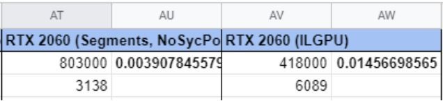
During our tests for this chapter, we used two different C# (MSIL) -> Cuda PTX compilers. Initially, we favored the ILGPU project (https://github.com/m4rs-mt/ILGPU) which is open source and promises cross-platform support in future releases. Unfortunately, performance results were underwhelming so we later switched to Tandem compiler which managed to better utilize the HW and yields 3.7x better performance. We used Tandem’s numbers in this chapter as it better represents the capabilities of the GPGPU and tested HW, but it’s currently not licensed so we can share sources only for ILGPU version of the GPU Badger.
ILGPU notes
Pros
Works on NVidia and AMD GPUs
Cuda
OpenCL
Extensive APIs and syntax sugar
All backends are nicely hidden under platform agnostic API
There are handy helpers for common stuff
For Unreal RHI we’ll need to implement our own backend from scratch
Out of the box ready GPU algorithms
There is sister lib with GPU optimized algorithms
Nature, quality and usability needs to be further evaluated
Nice samples
Helped me to get started quite smoothly
Cons
No console support
Poor performance
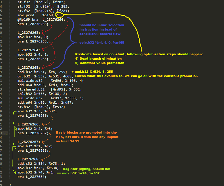
By comparing output assembly (SASS) to Tandem’s output and hand-tweaking the source to match Tandem’s output I managed to improve the ILGPU’s performance to be only ~2x slower compared to Tandem, but couldn’t get any better than that. This is generally possible only when you have another (better) compiler that you can use as a cheat sheet for comparison, blind assembly optimization in any reasonable timeframe is not an option.
Weak optimizer
Heavy on registers => Forced spilling and/or low occupancy
No constant value promotion & propagation => Burning cycles with meaningless instructions
No dead code elimination => Adds jumps, introduces instruction fetch stalls
Limited instruction set usage => More instructions means longer runtime
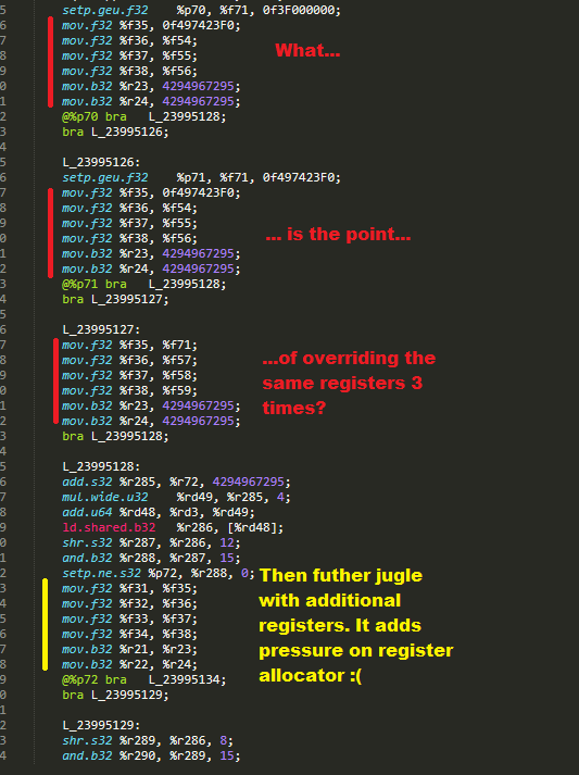
Questionable codegen
By hand-tweaking the source code and evaluating output SASS I could get rid of some issues (overloaded FP64 APU, ordering of hot and cold blocks, partially register overuse), but I’m unable to fix these:
2x more SASS instructions; 1 instruction ~ 1 clock cycle => 2x slower
3x more branch instructions => Increased thread divergence
17 calls (using some fancy math instructions for div and sqrt, fast math flags didn’t get rid of all calls)
Supports only basic compute kernels, no support for “runtime features”
No Dynamic parallelism (GPU spawning work for itself)
No Cooperative groups (Fine-grained thread synchronization and co-operation)
Missing some essential APIs (should not be that hard to fork the lib and implement)
Memory pinning
Launch graphs
Sometimes overkill abstractions
3 layers just to wrap IntPtr 🙂 => Virtual calls, we’ll pay for that
C# coverage is limited
No foreach
No StructLayout
No nested functions
No try/finally
No using statement and using variables
No stackalloc
(This is expected) No managed objects, arrays, lambdas, …